Block 3: Life is Continuous
Regression with multiple predictors
Mediation effects
Interaction effects
Chi-square
Bayes!
In this lecture we aim to:
Repeat some regression
Look at multiple predictors
Show these in JASP
Reading: Chapter 8 (§8.9–8.16)
Multiple regression
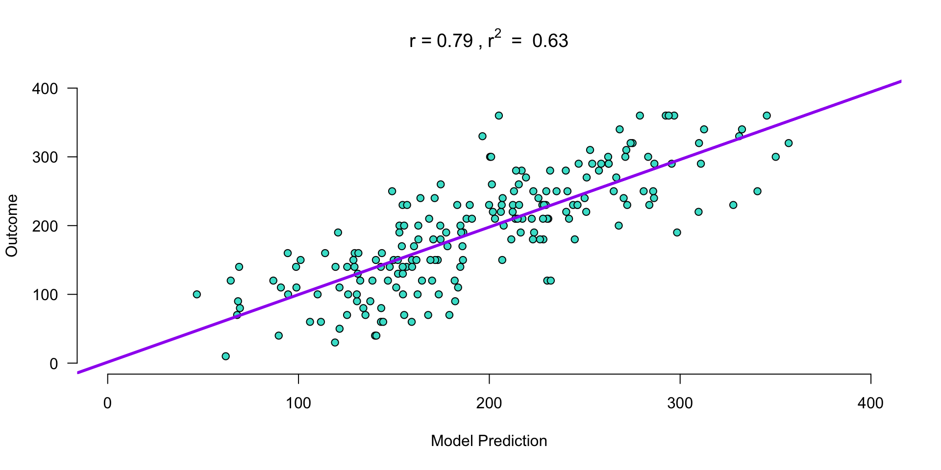
\(\LARGE{\text{outcome} = \text{model prediction} + \text{error}}\)
In statistics, linear regression is a linear approach for modeling the relationship between a scalar dependent variable y and one or more explanatory variables denoted X.
\(\LARGE{Y_i = \beta_0 + \beta_1 X_{1i} + \beta_2 X_{2i} + \dotso + \beta_n X_{ni} + \epsilon_i}\)
In linear regression, the relationships are modeled using linear predictor functions whose unknown model parameters \(\beta\) ’s are estimated from the data.
Source: wikipedia
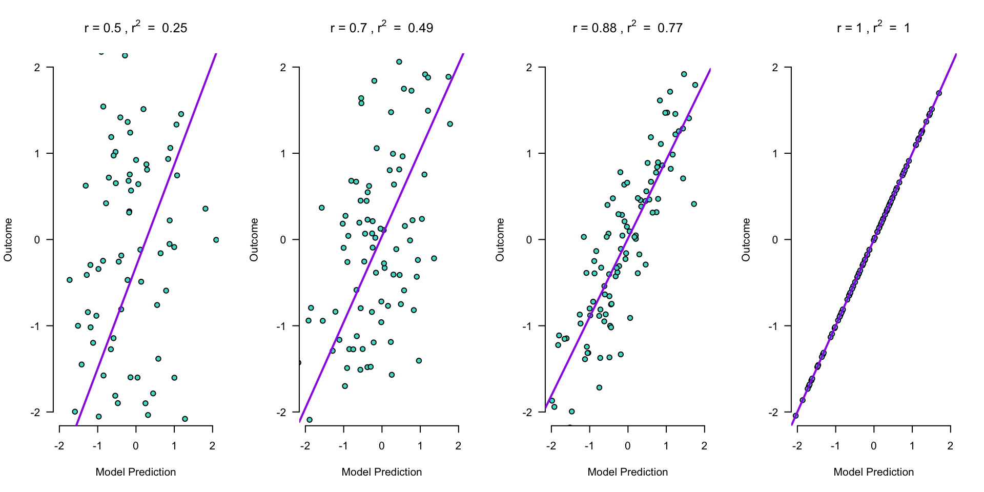
Outcome vs Model Prediction
Assumptions
A selection from Field (8.3 Bias in linear models):
For simple regression
Sensitivity
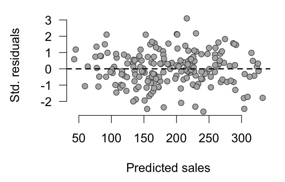
Homoscedasticity
See here for further illustration
Linearity
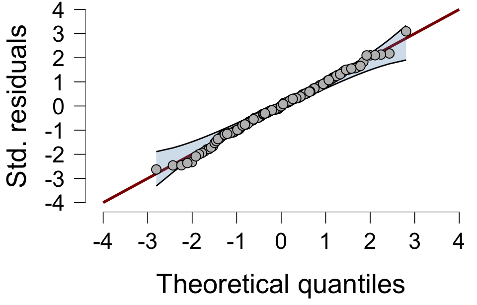
Normality
Additionally, for multiple regression
Multicollinearity (Section 8.9)
Homoscedasticity
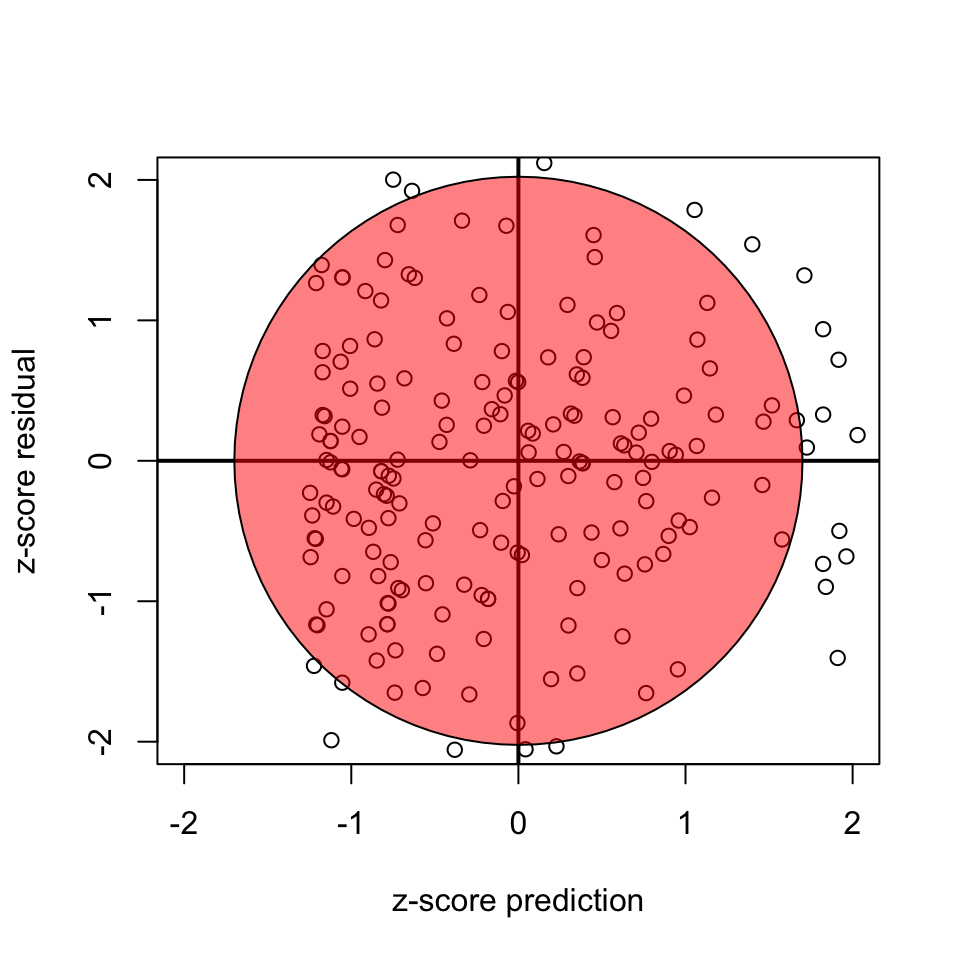
Variance of residuals should be equal across all expected values
Look at scatterplot of residuals vs. predicted values. Ideally it’s an uncorrelated, round cloud
For examples of violations, see here
After the analysis is complete because it’s based on the residuals
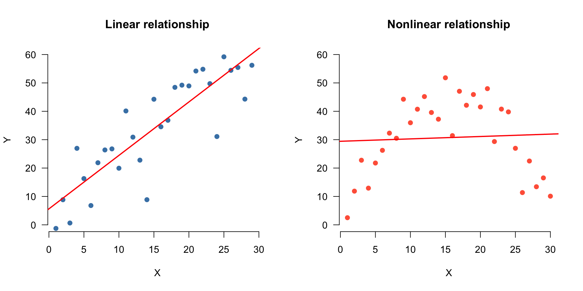
Linearity
For the linearity assumption to hold, the predictors must have a linear relation to the outcome variable.
This can be checked through:
Correlations
Matrix scatterplot with predictors and outcome variable
Robust alternative: bootstrap
Assumptions in doubt? Confidence intervals and \(p\) -values may be off
Bootstrap the coefficients (Section 8.12)
Statistics → Coefficients → From 5000 bootstraps
Output: Bootstrap Coefficients table
More robust methods (e.g., winsorizing, Section 6.10.7)
Robust Statistics module (WRS2)Not exam material
Example
Predict album sales (1,000 copies) based on airplay (no. plays) and adverts ($1,000).
Link
Regression model
Predict album sales based on airplay and adverts.
\[{sales}_i = b_0 + b_1 {airplay}_i + b_2 {adverts}_i + \epsilon_i\]
<- lm (sales ~ airplay + adverts, data = data)
What is the model?
The beta coefficients are:
\(b_0\) (intercept) = 41.12\(b_1\) = 3.59\(b_2\) = 0.09.
How to visualize??
When we plot 1 predictors + DV, we plot in 2 dimensions, and we summarize the relationship by a line
When we plot 2 predictors + DV, we plot in 3 dimensions, and we summarize the relationship by a plane
… ???
Cool visualization app for 2 predictors
What are the predicted values based on this model
\(\widehat{\text{album sales}} = b_0 + b_1 \text{airplay} + b_2 \text{adverts}\)
<- b.0 + b.1 * airplay + b.2 * adverts
\(\text{model prediction} = \widehat{\text{album sales}}\)
Apply regression model
\(\widehat{\text{album sales}} = b_0 + b_1 \text{airplay} + b_2 \text{adverts}\)
\(\widehat{\text{album sales}} = 41.12 + 3.59 \times \text{airplay} + 0.09 \times \text{adverts} = 196.413\)
How far are we off?
<- sales - predicted.sales
Outcome = Model Prediction + Error
Is that true?
== predicted.sales + error
  [1] TRUE TRUE TRUE TRUE TRUE TRUE TRUE TRUE TRUE TRUE TRUE TRUE TRUE TRUE TRUE
 [16] TRUE TRUE TRUE TRUE TRUE TRUE TRUE TRUE TRUE TRUE TRUE TRUE TRUE TRUE TRUE
 [31] TRUE TRUE TRUE TRUE TRUE TRUE TRUE TRUE TRUE TRUE TRUE TRUE TRUE TRUE TRUE
 [46] TRUE TRUE TRUE TRUE TRUE TRUE TRUE TRUE TRUE TRUE TRUE TRUE TRUE TRUE TRUE
 [61] TRUE TRUE TRUE TRUE TRUE TRUE TRUE TRUE TRUE TRUE TRUE TRUE TRUE TRUE TRUE
 [76] TRUE TRUE TRUE TRUE TRUE TRUE TRUE TRUE TRUE TRUE TRUE TRUE TRUE TRUE TRUE
 [91] TRUE TRUE TRUE TRUE TRUE TRUE TRUE TRUE TRUE TRUE TRUE TRUE TRUE TRUE TRUE
[106] TRUE TRUE TRUE TRUE TRUE TRUE TRUE TRUE TRUE TRUE TRUE TRUE TRUE TRUE TRUE
[121] TRUE TRUE TRUE TRUE TRUE TRUE TRUE TRUE TRUE TRUE TRUE TRUE TRUE TRUE TRUE
[136] TRUE TRUE TRUE TRUE TRUE TRUE TRUE TRUE TRUE TRUE TRUE TRUE TRUE TRUE TRUE
[151] TRUE TRUE TRUE TRUE TRUE TRUE TRUE TRUE TRUE TRUE TRUE TRUE TRUE TRUE TRUE
[166] TRUE TRUE TRUE TRUE TRUE TRUE TRUE TRUE TRUE TRUE TRUE TRUE TRUE TRUE TRUE
[181] TRUE TRUE TRUE TRUE TRUE TRUE TRUE TRUE TRUE TRUE TRUE TRUE TRUE TRUE TRUE
[196] TRUE TRUE TRUE TRUE TRUE
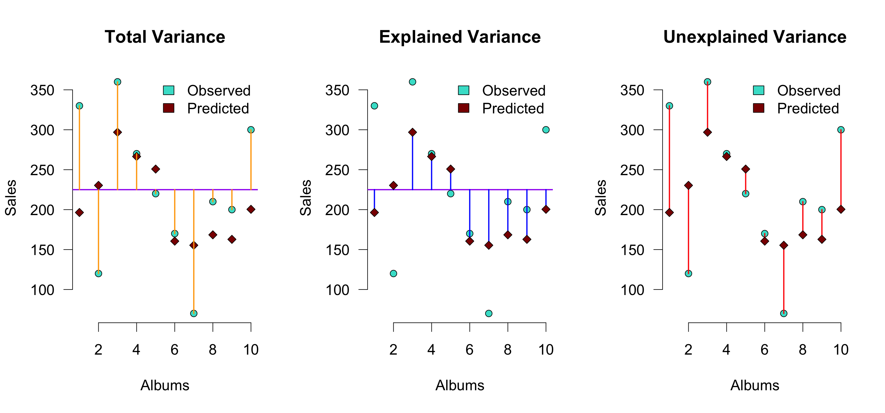
Visual (subset of 10 albums)
\(r^2\) is the proportion of blue to orange , while \(1 - r^2\) is the proportion of red to orange
Explained variance
The explained variance is the deviation of the estimated model outcome compared to the grand mean.
To get a percentage of explained variance, it must be compared to the total variance. In terms of squares:
\(\frac{{SS}_{model}}{{SS}_{total}}\)
We also call this: \(r^2\) or \(R^2\) .
Why?
<- cor (sales, predicted.sales)^ 2
Explained variance